
Say you’re running an LLM, and you want to make the most out of whatever GPUs you can get your hands on.
When you don’t train the model yourself, one of the best techniques at your disposal to optimize inference is post-training quantization (PTQ). Specifically, mixed-precision quantization of model weights and activations.
The goal is to make parts of the model smaller, and sacrifice as little of its quality as possible. Think of it like the machine learning equivalent of poking more holes in a slice of Swiss cheese. No one would notice a few more tiny holes, but if you dare to poke too liberally… people will have questions.
In this post we sketch out the techniques we used to improve upon the official FP8 checkpoint of GLM-5.3 Flash, reducing memory footprint by ~10% with only a ~3% drop in output quality on our internal benchmarks.
Aside
If you’re unfamiliar with LLM quantization, this post will be confusing. There are a few learning resources at the bottom of this post.
1 Inspiration
In the past months, two PTQ-adjacent announcements caught our attention.
First, Baseten published a paper that describes how to predict which combinations of an LLM’s layers are least likely to degrade quality when quantized. Meaning, we can quantize a subset of layers with only minimal damage to the model’s intelligence, and leave the layers most important for output quality completely untouched.
Second, Tencent touted their use of an ultracompact quantization technique called “Sherry” (or STQ1_0), which reduced the size of their flagship model, Hy4-preview, from 1.5T to 214GB, and impacted model quality by only a few percentage points.

Now, in all likelihood, Hy4-preview employed quantization-aware training (QAT) to make this staggering reduction in model size possible. But that doesn’t mean it can’t be helpful on other models.
In the spirit of Science, we thought it would be interesting to marry these two approaches and try STQ1_0 quantization for a selection of layers in a house-favorite model: GLM-5.3 Flash. The experiment went as follows:
Calibrate the transformer block activations with a dataset.
Fit a predictor for layer sensitivity, using damage measurements from random permutations of quantized layers.
Verify the predictor against holdouts and alternative predictors.
Evaluate the effects of STQ variants when quantizing 8, 16 and 24 layers.
2 Shy experts and a preponderance of datasets
Calibrating the activations didn’t require much finesse. We simply sourced a dataset with a mix of agent-like requests (tool calls, code, etc.) and ran it through the model.
The only bump in the road was that the dataset needed to hit each of the model’s 288 routed experts, but some experts wound up being a little shy. Meaning, the first few datasets we tried for calibration didn’t see every expert light up.
So, we doubled the size of the dataset and voilà. We were calibrated.
From there, we gathered another dataset of precomputed STQ1_0 weights and calibrated activations for all 45 layers of the model (3 dense and 42 MoE).
But then, would you believe it, we needed yet another dataset, this time ~150 distinct, random permutations of quantized layers, with a measurement of how much damage each permutation caused relative to a higher precision control. Finally, we had everything we needed to fit a predictor for layer sensitivity.
3 Small, but slow
Creating the data we would use in our predictor was a slow, slow process. So slow as to arouse suspicion.
When profiled, end-to-end latency for requests to the STQ models was 7–12× slower than the off-the-shelf FP8 checkpoint. As it were, the inference code for the experiment lacked some premature optimizations that would have been, in fact, not premature at all.
We had started with a naive implementation, and fixing the slowness of that naivety meant taking a detour into kernel-land. Tencent graciously published the patch they wrote for llama.cpp to get STQ1_0 running smoothly. Using that as inspiration, we got enough of a speedup to run the rest of the experiment at a reasonable clip.
After sampling 150 or so permutations of quantized layers, we fit a few different damage predictors and tested them against both random sampling and each other. The two clear winners were the coverage and additive models of layer sensitivity.
The coverage model, which was the core of the Baseten paper, predicts the damage caused by quantization by assuming a maximum of total possible damage, c. Each quantized layer eats a percentage, not a fixed amount, of whatever part of c the other layers haven’t consumed yet.
Think of c as a pie. Say layer aᵢ likes to eat 5% of the pie and layer aᵢ₊₁ invariably indulges in 8%. If aᵢ already ate its 5%, then aᵢ₊₁ eats 8% of 0.95 c.

When S is a set of quantized layers, we get a predictor like so:

The additive model is a simpler approximation of damage. It avoids modeling interactions between layers, and just reflects the idea that each layer does a predictable amount of damage when quantized:

Aside
The intercept term b turns out to be very important. Remove the intercept parameter, and the additive model is hot trash.
Both of these models kept prediction error acceptable when extrapolated, and chose categorically better mixed-precision layer configurations than random selection.
Aside
In contrast to the Baseten paper, which put forward the coverage model, we did not find a statistically significant improvement of the coverage model over its additive counterpart.
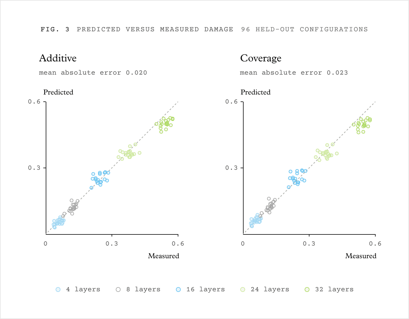
Each point is one of 96 unseen layer combinations, evaluated on final held-out text. Damage is the equal-weight mean increase in prose and code cross-entropy versus BF16, in nats per target token. The coverage model approaches an additive limit; this plot does not establish saturation or task-quality retention.
With our predictor more or less validated, we treated its coefficients as a ranking of layer sensitivity, and selected a few mixed-precision quantizations for evaluation.
4 Budgeting
We set three budgets, targeting a reduction in memory of roughly 30%, 20% and 10%, with lightweight quality checks to make sure the model still, at a bare minimum, returned sensible outputs. After that, internal benchmarks were the judge of how noticeably we’d disturbed the model.
STQ layers | Approximate memory-reduction target |
|---|---|
8 | 10% |
16 | 20% |
24 | 30% |
Rounded budget targets for this post, not measured savings. Actual GPU memory savings depend on the baseline checkpoint, cache policy and serving implementation.
At ~30%, quality fell sharply. In some cases the model failed to emit proper tokens to demarcate thinking blocks. We poked too many holes in the proverbial Swiss cheese, and were left with a pile of crumbs. Perhaps suitable for a mouse, but disappointing for a human.
At ~20%, we saw encouraging pass rates, with a peculiar side effect: the model spent 3–5× as much time thinking. The overall effect was more work done per task, which we considered a failure.
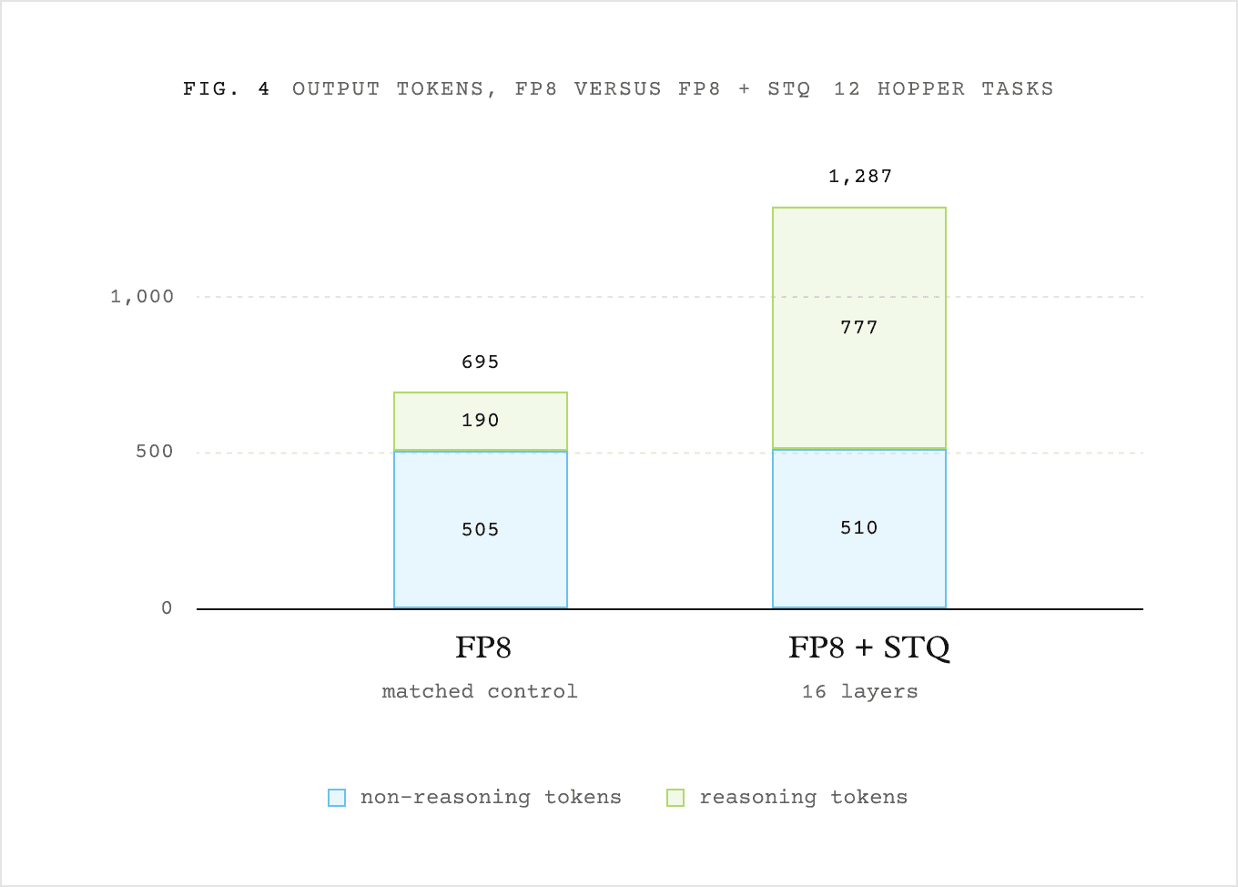
Totals across the same 12 Hopper tasks, one response per task per arm. FP8 is the matched FP8 control, not the optimised arm. These are token counts, not time measurements.
At ~10%, the quantized layers hit a sweet spot. Not only did we achieve a practically equivalent pass rate to the FP8 checkpoint, it left us enough headroom in the node to increase batch size, yielding higher throughput for the shape of traffic we support.
5 Conclusions
Testing and predicting layer sensitivity is a useful exercise when you need to craft your own mixed-precision quant under a budget. There is an initial investment in the experimentation setup, but after that it can largely be managed by an agent while you tackle other work.
The hidden cost is that while clever, low-bit quantization techniques like Sherry help to fit a large model on constrained hardware, they come with added engineering effort once you enter a datacenter. There, where the model may already fit and kernels are already optimized for more widely used quants, it takes a touch of low-level tinkering to get robust performance when serving the model.